Anomaly Detection with R, H20 and MinIO

Anomaly detection is an area of Machine Learning that is powerful and applicable to many domains. It can also be a bit of a black box and is often confused with classification - I’ve heard it described as “classifying” instances into “good” or “bad”. I think it’s worth opening the black box and taking a look inside to gain some clarification.

For this article we will use the MNIST dataset. If you are unfamiliar with MNIST it can be thought of as the “Hello World” of machine learning for classification problems and anomaly detection problems. The dataset consists of digitized hand-written numerical digits contributed by Census Bureau workers (the generally readable digits) and high school students (the less recognizable digits). Given this mix, it lends itself to being a standard dataset against which to test a wide variety of machine learning models as well as pre-processing steps for the data. If you’d like to learn more, please see the raw datasets and a summary of some of the studies and publications around the MNIST dataset.

For part one of this series we will use H2O anomaly detection and MinIO to store, process, and identify anomalies in the data set. This series is a follow-up to my previous post, Machine Learning Using H20, R and MinIO.

The MNIST data set consists of digitized hand-written digits with some preprocessing already applied. Preprocessing is described as follows: “The original black and white (bilevel) images from NIST were size normalized to fit in a 20x20 pixel box while preserving their aspect ratio. The resulting images contain gray levels as a result of the anti-aliasing technique used by the normalization algorithm. the images were centered in a 28x28 image by computing the center of mass of the pixels, and translating the image so as to position this point at the center of the 28x28 field.”

The digits generally look like this:

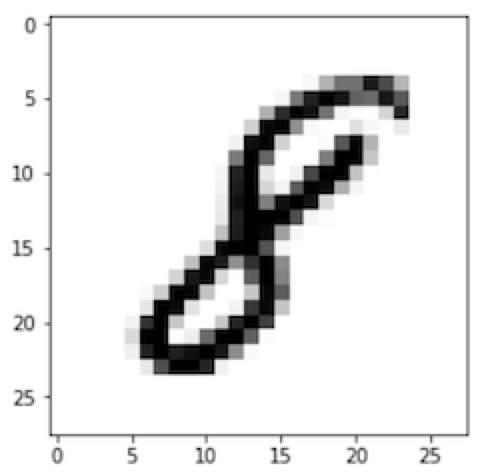
And are converted into a vector of gray-scale pixel values in the range of 0 to 255.

It’s important to realize that there are multiple ways this domain data (the hand-written numeral) could have been represented for modeling. A grid of gray-scale values seems intuitive (a bitmap), but has implications for the application of anomaly detection or any other machine learning approach to the real world data. There are a number of ways this domain data could have been transformed into the numerical vectors required for machine learning approaches, some would work better, some would work worse for a given modeling approach. There is no single right answer for how best to represent domain data for modeling, and this is important. There is also no right answer for how best to preprocess the representation.

LeCun, Cortez, and Burges state that “With some classification methods (particularly template-based methods, such as SVM and K-nearest neighbors), the error rate improves when the digits are centered by bounding box rather than center of mass.”

Looking through the summary of the studies referenced above, there are a number of additional pre-processing steps that many of the studies used to enhance performance.

The implications for designing, conducting and analyzing data science experiments are dramatic. The statistical and numerical modeling of the domain data for any given problem in any given domain is not immediately obvious. Even the experts agree that this is tricky stuff. Think about it - if we as humans understood the relationship in the data well enough to be able to identify a-priori how best to represent it, then it is likely we would have already built systems to accurately model that relationship. Problems and modeling that truly require ML are generally very messy and intricate. Determining how to curate the data and transform it into a form that the model can understand in order to uncover the intrinsic relationships hidden within the raw data is almost always vastly more difficult than making the Python or R library calls needed to train the model.

Enough theory and talk; time to code.

H20, R and MinIO for Anomaly Detection

There are a ton of tutorials that cover MNIST in virtually every language under the sun, as well as every machine learning platform. Personally, I like H2O. I find it fast, easy to manage and use, and very complete with the capabilities it offers. I also like working in R. I find R to be the most intuitive for me when I work with data and Machine Learning. Combining these two with MinIO Object Storage creates a very powerful platform for data scientists.

If you are not familiar with H2O, it is an open source distributed in-memory machine learning environment. I described H20 more fully in an earlier post, Machine Learning Using H20, R and MinIO.

If you are not familiar with the R programming language for statistical computing, it is used by statisticians and data miners for data analysis. I described R more fully in an earlier post, MinIO and Apache Arrow Using R. I find R to be rather intuitive when I am working with data, data analysis and machine learning.

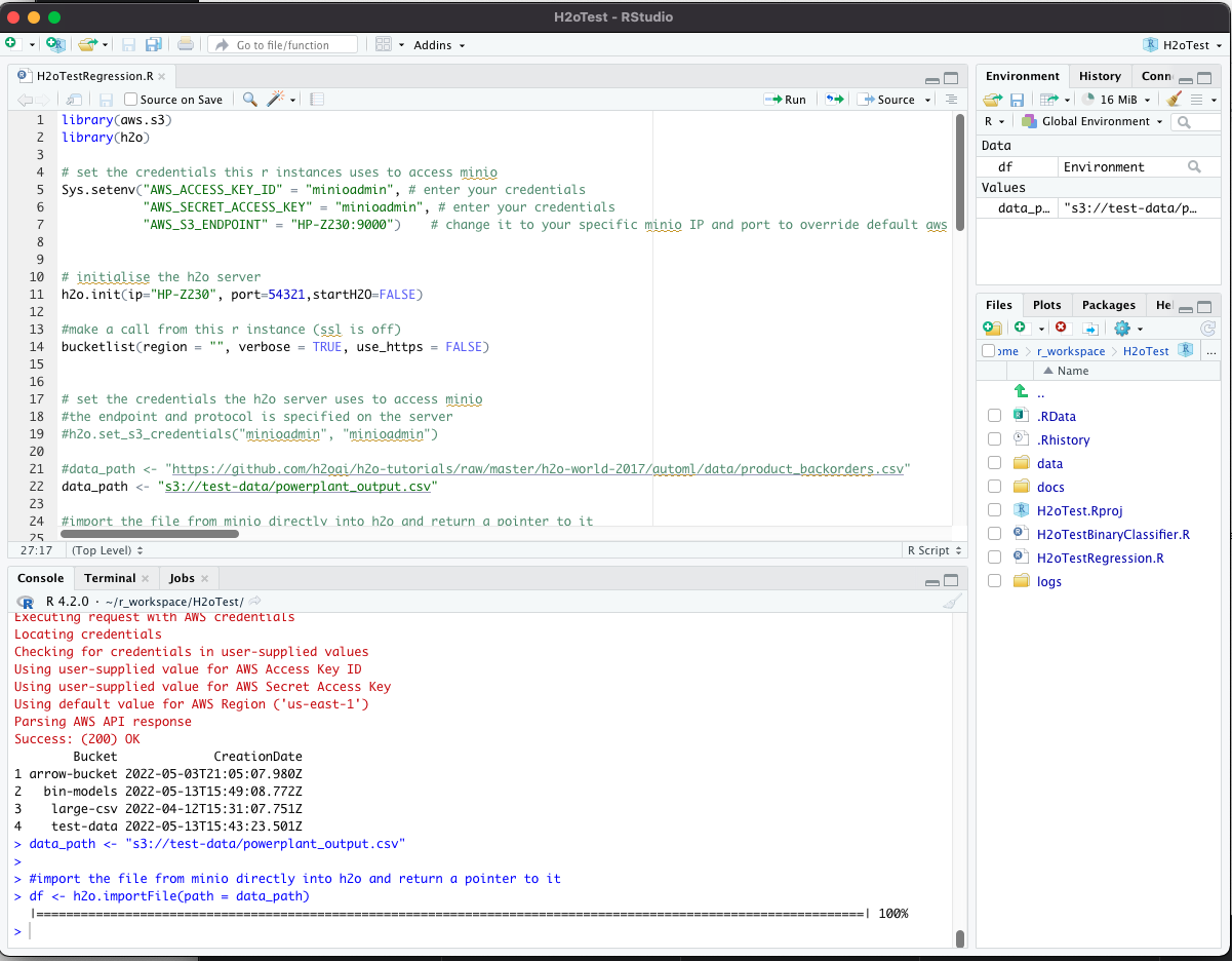
The R language has a companion IDE called RStudio, which I will use for this development: https://www.rstudio.com/. The IDE generally looks like this:

MinIO is high-performance software-defined S3 compatible object storage, making it a powerful and flexible replacement for Amazon S3.

If you want to follow along please install R and RStudio, have access to an H2O cluster, and if you aren’t already running MinIO, please download and install it. In addition, please download and install the aws.s3 R library.

Let’s Get Coding!

In this blog post, I’m going to set up H2O, R, and MinIO to perform anomaly detection using the built-in capabilities of H2O. In my previous post, Machine Learning Using H20, R and MinIO we did this with an external H2O cluster, in this post we will launch H2O from within R.

I start by downloading the raw files to my local drive. These raw files are in a specific binary format and need to be read in, converted, and written out in tabular format for use. I anticipate running many models and preprocessing approaches against these files, so I will convert and store them in a commonly API-accessible MinIO object store.

First load the required libraries and credentials, then initialize the H20 and load the MNIST data. Please note that some of the code below for showing a digit and loading and processing the binary MNIST files is taken directly from David Dalpiaz's code on github. David is Teaching Assistant Professor for the Department of Statistics at The University of Illinois at Urbana-Champaign.

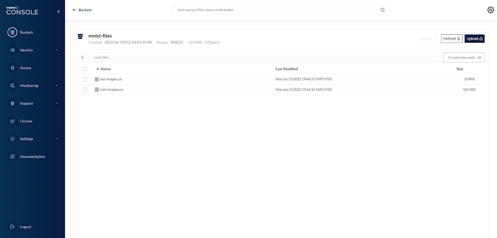
Now that the data is loaded and transformed, we can save it to MinIO. Using the MinIO Console, I created a new bucket called mnist-files, and wrote the files to that bucket. This is the end of getting the data ready for modeling:

Returning to MinIO Console, we see that the files were written to our bucket.

What Exactly is an Anomaly?

Once the data is stored centrally in a format that H2O can read, we can start using H2O’s anomaly detection capabilities to analyze it. But first, what exactly are anomalies and how does an auto-encoder “detect” them?

If we take a 3-layer neural network with input and output vectors of identical lengths and feed something representing “information” (usually pixels of an image, but it can be any type of information) into the input vector and train the network to produce the identical results on the output vector, we will have taught the network to approximate the identity function (f-hat() approximates f(), which is the identity function since we used the input vector as the ground truth for the supervised training)

If the middle layer has fewer neurons than the input vector, then we could view the weight matrix between the input and middle layers as “compressing” the information to store it in the “more narrow” middle layer. We could also view the weight matrix between the middle layer and the output layer as uncompressing or reconstructing the information back to it’s original value. If we successfully train the network to convergence with a low enough error rate, we can then break the network into two pieces - compression and reconstruction - and use them separately. Theoretically, we could compress lots of data using the compression weight matrix and store the values from the middle layer neurons as the “compressed” version of the information. We could then reconstruct the original information using the weight matrix from the middle layer to the output layer. This approach works for deep learning networks as well - ones with more than one hidden layer.

Brilliant! One catch though - well , maybe two….

1. We need to be able to train the network to a very small error rate (often expressed as the Mean Squared Error - MSE - between the ground truth vector (which in this case is the same as the input vector) and the predicted vector that the model produces during training to closely approximate the identity function. MSE would need to be low enough so that when we reconstruct a given piece of information it won’t be exact, but it will be close enough that there won’t be confusion as to what it is.
2. We must also train the model on most, if not all, of the information that would be seen by the system in the future. The model has to be able to compress and reconstruct everything we hope to ever use it on.
   

I first encountered the approach of using a neural network with identical input and output vector lengths and training it on identical vectors of input and ground truth in the book “Neurocomputing “ by Robert Hecht-Nielsen, published in 1990. In the book, the author cites a paper by Cottrel, Munro, and Zipser from 1986 describing this approach. To my knowledge this approach isn’t used much for compression outside of possibly medical imagery since less costly processes can achieve similar results on a wider range of data. At the time (1990), the term “autoencoder” didn’t exist, nor did the use of this architecture for anomaly detection as far as I can tell.

At some point someone realized (not sure on the history of this) that there was another use for this architecture. That second caveat above - about having to train the network on all the information the model would see when run to achieve a low MSE - could be seen differently. It could be viewed as data that the model had been previously trained on would have a low MSE between the input vector (the data coming in ) and the output vector (the prediction of the model) when it was executed. And data that the model had not been trained on would likely have a larger MSE. The MSE could therefore be used to identify whether the data was “similar” to the training data - and the autoencoder for anomaly detection was born!

Since the autoencoder is trained on a set of data to a low MSE, if we run the autoencoder on new data and it reports a low MSE, then we know the new data should be similar to the data used in training - it’s “normal”. If we run the auto-encoder on new data and it results in a high MSE, then it is dissimilar to the data the model was trained on and could be considered “abnormal”. We generally assume that “abnormal” equates to “bad”, but this isn’t the case - “abnormal” only means that the data we ran through the auto-encoder exists in the multidimensional space of the input vector at some distance from where the training examples exist. It isn’t “bad”, it’s just “different”. For example, a company having a very, very profitable quarter might be “abnormal”, but it’s not subjectively “bad”.

It’s important to remember that anomaly detection doesn’t provide an indication of “good” or “bad”, and therefore is usually followed by the use of a classification model to assign “good” or “bad” to the anomalies (or some larger set of factor values that the classifier learns through supervised learning).

To sum that up, an anomaly is an occurrence of input that when passed through a properly trained auto-encoder results in a high MSE between what the auto-encoder predicts and the ground truth (the input vector in this case). This high MSE indicates the likelihood of the input vector not being similar to the examples the autoencoder was trained on. It is different in some meaningful way - it is an anomaly. Not good, not bad, just meaningfully different from the data the autoencoder was trained on.

Enough jabbering already, back to code.

Working with Data

We wrote the data to a common MinIO repository so that we could have H2O read the data from there directly and not be required to have the data pass through the R process running locally. Below, the paths are set up, the data is loaded into H2O running on the server directly from the MinIO store, and converted into the H2O preferred binary representation.

Please note that much of the code below is adapted from the h2o-r deep-learning repository section about anomaly detection tests:

Once the data is loaded in H2O we can begin to manipulate it. Remember that the form of the data is one row per written numeral, with 28 x 28 gray-scale pixel values used as the predictors (784 values in the first 784 columns) and one response - a 10 value factor indicating the numeric value that the handwritten image represents - 0 to 9 - in column 785. We assign those:

Since auto-encoders use the input vector (the predictors) as the response, we have no use for the values in column 785. If we were using this data for a prediction model, that column would be the ground truth for the training and testing set. In our case we can remove it:

In addition, let’s leverage some helper functions for visualizing the digits:

Since the data has just been loaded into H2O, it’s a single call to easily train a basic auto-encoder using the capabilities of the H2O platform. A deeper explanation of the parameters of this call are for another day.

Remember that the input vector is also the ground truth for the auto-encoder process, so there is a single call in H2O that runs the test data through the specified model and computes the MSE per row. This is usually all you want to know - for a given row, is the MSE is “too high”, indicating that the instance of the data in that row is an anomaly:

For the purposes of demonstration, let’s take this a step further. The code below will display the digits associated with low and high reconstruction errors:

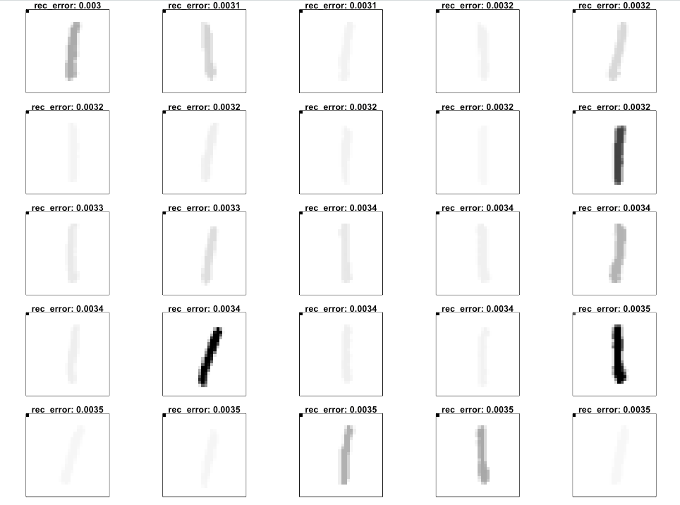
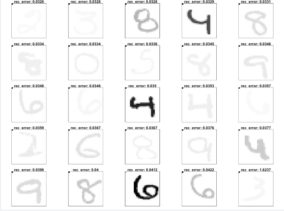
From this we see that the lowest reconstruction MSE comes from well written examples of the numeral “1” - the simplest digit. The highest MSE comes from slightly irregularly written digits that are more complicated - “8”, “4”, “6”, and “2”.

It makes sense that the numerals with the highest variation are in the set of those with high reconstruction error. In my next blog post, I’ll show you how to apply this framework to something more real-world - Apache web server log access files.

A note about results, results from H2O are not reproducible if they are run on more than a single core. The results and performance metrics may vary slightly each time you train the deep learning model. The implementation in H2O uses a technique called “Hogwild!” which increases the speed of training at the cost of reproducibility on multiple cores. If you want reproducible results you will need to restrict H2O to run on a single core and make sure to use a seed in the h2o.deeplearning call as well as setting reproducible=TRUE.

Getting Started with Anomaly Detection

MNIST is a well-known standardized dataset that is used for classification model development and testing as well as anomaly detection development and testing. There are a number of ways to perform anomaly detection in data, and autoencoders are frequently used and fairly simple to understand. In this process, the input vector for the training examples is also used as the ground truth for the training and the result is that the model is trained to learn the identify function for the training examples. Afterwards, the model can run against new data to determine how “close” it is to the training data in the multidimensional input vector space - the magnitude of the MSE is an indication of “normality” and “abnormality”. Typically this anomaly detection step feeds into a classifier (that has been trained using supervised training) that more precisely classifies the instance as appropriate for the problem domain.

The technologies highlighted in this blog post - R, H20 and MinIO - form a powerful and speedy ML toolbox. This tutorial provided an example of anomaly detection and provided a hefty dose of theory - all good things to learn before the follow-up blog post about anomaly detection over Apache access logs.

Download MinIO and build your ML toolkit today. If you have any questions, please send us an email at hello@min.io, or join the MinIO slack channel and ask away.