MinIO and Apache Arrow Using R

Brian Costa Brian Costa on Apache Arrow 17 May 2022

Arrow here, Arrow there, Arrow everywhere. Seems like currently you can't swing a dead cat without hitting an article or blog post about Apache Arrow. Most seem to be addressing a developer audience and are based on a Python and Spark style development platform. Today I’m going to write about using Apache Arrow with MinIO from the R programming language.

If you are not familiar with R (from Wikipedia):

“R is a programming language for statistical computing and graphics supported by the R Core Team and the R Foundation for Statistical Computing. Created by statisticians Ross Ihaka and Robert Gentleman, R is used among data miners and statisticians for data analysis and developing statistical software. Users have created packages to augment the functions of the R language.”

I find R to be the most intuitive for me when I am working with data, data analysis and machine learning.

MinIO is high-performance software-defined S3 compatible object storage, making it a powerful and flexible replacement for Amazon S3.

And, finally, if you are not familiar with Apache Arrow (from the website):

“Apache Arrow defines a language-independent columnar memory format for flat and hierarchical data, organized for efficient analytic operations on modern hardware like CPUs and GPUs.”

The combination of Arrow, R and MinIO forms a very powerful platform for data analysis on large data sets. I will be working with a 5 million row csv file of randomly generated sales data from “E for Excel”.

Please be aware this data is fictitious. E for Excel prominently states: “Disclaimer – The datasets are generated through random logic in VBA. These are not real sales data and should not be used for any other purpose other than testing.”

I chose this dataset because it is fairly simple in structure and is large enough to capture some timing metrics on the analytics processing.

The R language has a companion IDE called RStudio, which I will use for this development. If you want to follow along please install R and RStudio, and have access to a MinIO cluster. If you aren’t already running MinIO and mc, the MinIO client, please download and install them.

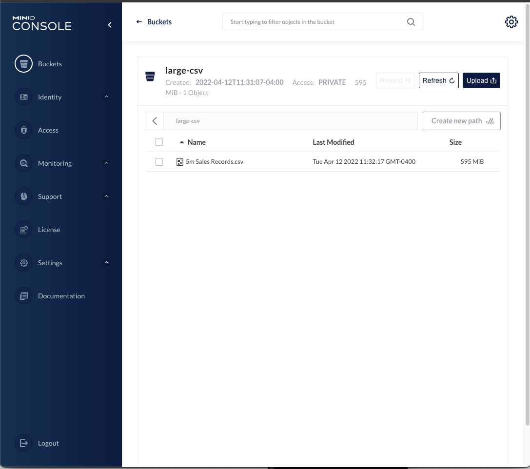
I started by downloading the sales data to a local directory on my machine, and copying it to a bucket on MinIO. Copying the file to MinIO can be accomplished using the MinIO command line tool mc, or uploading the file from within the MinIO console. I created a bucket called large-csv and uploaded the 5m Sales Records.csv file to it from within the console. This is the starting point for the work we will do.

There are a number of resources available on the web for working with MinIO from R, as well as working with Apache Arrow from within R. Here are two links I found useful in putting these things together:

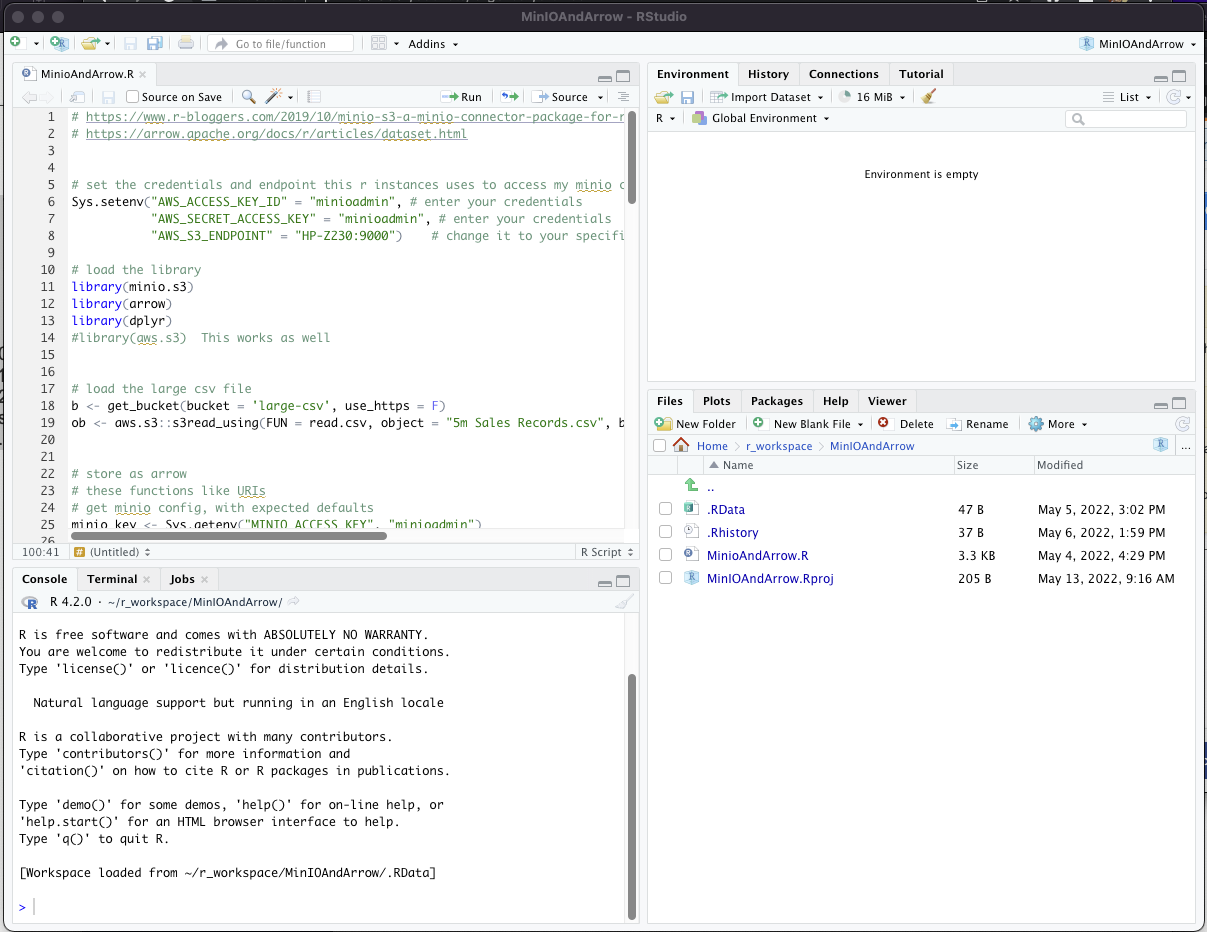
Now onto the coding. As I mentioned I’m working in R from within R studio. R studio is a common IDE for working with R and looks like this:

I’m going to paste the code in this article in sections.

This is the beginning. It’s the code to set the environment and load the required libraries into the R. Notice the use of the environment for passing the credentials and endpoint. There are several ways to make these values available to the libraries, including integrations with most IAM systems. For the purposes of demonstration this seemed the simplest:

# set the credentials and endpoint this r instances uses to access my minio cluster
Sys.setenv("AWS_ACCESS_KEY_ID" = "minioadmin", # enter your credentials
"AWS_SECRET_ACCESS_KEY" = "minioadmin", # enter your credentials
"AWS_S3_ENDPOINT" = "HP-Z230:9000")  # change it to your specific minio IP and port to override default aws s3
# load the library
library(minio.s3)
library(arrow)
library(dplyr)
#library(aws.s3) This works as well

Next I’ve included the code necessary to read the large csv file from the bucket in MinIO. What I’ve done below requires that the entire csv fit into memory on this client. If your csv file is too large to fit into memory there are several ways to process the file in smaller chunks within a loop. The code below gets a handle to the bucket and reads the object.

# load the large csv file
b <- get_bucket(bucket = 'large-csv', use_https = F)
ob <- aws.s3::s3read_using(FUN = read.csv, object = "5m Sales Records.csv", bucket = b, opts = list(use_https = FALSE, region = ""))

Once we have the tabular data of the csv in an object, we will write it to another bucket in Arrow format. The Arrow libraries like URLs, so I’ve created a couple of functions to make constructing the URLs easier:

# these functions like URLs
# get minio config, with expected defaults
minio_key <- Sys.getenv("MINIO_ACCESS_KEY", "minioadmin")
minio_secret <- Sys.getenv("MINIO_SECRET_KEY", "minioadmin")
minio_host <- Sys.getenv("MINIO_HOST", "hp-z230")
minio_port <- Sys.getenv("MINIO_PORT", "9000")
minio_arrow_bucket <- Sys.getenv("MINIO_ARROW_BUCKET", "arrow-bucket")
# helper function for minio URIs
minio_path <- function(...) paste(minio_arrow_bucket, ..., sep = "/")
minio_uri <- function(...) {
template <- "s3://%s:%s@%s?scheme=http&endpoint_override=%s%s%s"
sprintf(template, minio_key, minio_secret, minio_path(...), minio_host, ":", minio_port)
}

The advantage of the Arrow format is that the data can be optimized for the anticipated queries that will subsequently be executed. Dplyr group_by is used to set the partitioning scheme. Partitioning, like setting useful indexes on a database, requires some idea of how the data will be queried or used. Partitioning imposes a cost as well as a benefit. There is a trade-off to be made and if one understands how the data is most often queried then the trade-off can be beneficial. For this example I’m going to assume the sales data is analyzed for a given country. If, on the other hand the data is most often analyzed by item type across countries, then this partitioning scheme probably won’t help. An attempt to partition by every column (just in case) defeats the benefit of the partitioning. Here is an explanation of the guidelines are from an article on using Arrow with R (https://arrow.apache.org/docs/r/articles/dataset.html):

Partitioning Performance Considerations

Partitioning datasets has two aspects that affect performance: it increases the number of files and it creates a directory structure around the files. Both of these have benefits as well as costs. Depending on the configuration and the size of your dataset, the costs can outweigh the benefits.

Because partitions split up the dataset into multiple files, partitioned datasets can be read and written with parallelism. However, each additional file adds a little overhead in processing for filesystem interaction. It also increases the overall dataset size since each file has some shared metadata. For example, each parquet file contains the schema and group-level statistics. The number of partitions is a floor for the number of files. If you partition a dataset by date with a year of data, you will have at least 365 files. If you further partition by another dimension with 1,000 unique values, you will have up to 365,000 files. This kind of partitioning often leads to small files that mostly consist of metadata.

Partitioned datasets create nested folder structures, and those allow us to prune which files are loaded in a scan. However, this adds overhead to discovering files in the dataset, as we’ll need to recursively “list directory” to find the data files.

Too fine partitions can cause problems here: partitioning a dataset by date for a year’s worth of data will require 365 list calls to find all the files; adding another column with cardinality 1,000 will make that 365,365 calls.

The most optimal partitioning layout will depend on your data, access patterns, and which systems will be reading the data. Most systems, including Arrow, should work across a range of file sizes and partitioning layouts, but there are extremes you should avoid. These guidelines can help avoid some known worst cases:

Avoid files smaller than 20MB and larger than 2GB.

Avoid partitioning layouts with more than 10,000 distinct partitions.

For file formats that have a notion of groups within a file, such as Parquet, similar guidelines apply. Row groups can provide parallelism when reading and allow data skipping based on statistics, but very small groups can cause metadata to be a significant portion of file size. Arrow’s file writer provides sensible defaults for group sizing in most cases.”

Given my assumption that the data will be analyzed within a country this is the code to write the Arrow format dataset to a different bucket in MinIO.

# partition by the "Country" column - we typically analyze by country
ob %>%
group_by(Country) %>%
write_dataset(minio_uri("sales-data"), format = "arrow" )

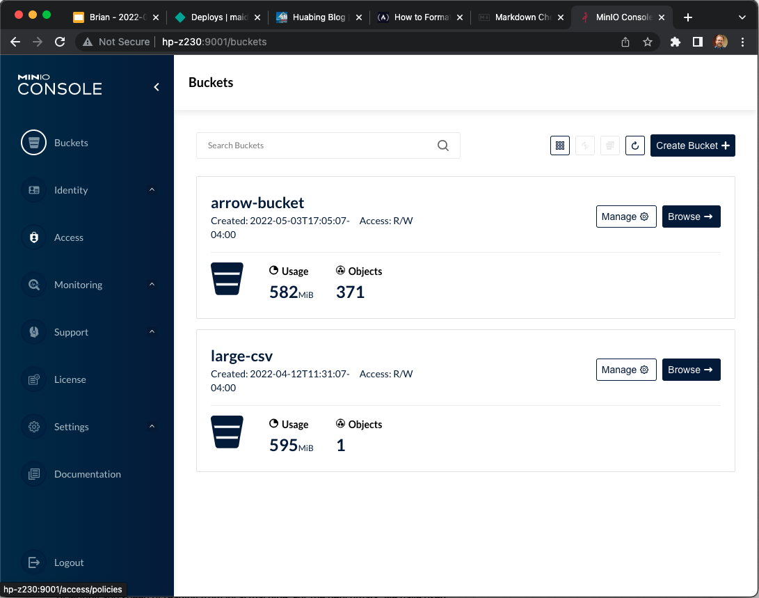
If we look at the results we see the creation of multiple files to support the partitioning.

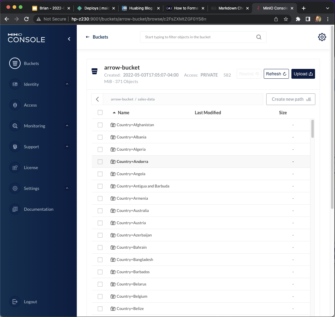
And if we look at the content of the arrow-bucket we see that the data has been partitioned by Country, as expected:

And that’s all the code to read the .csv file and store the dataset in Arrow format on MinIO. Next we will be opening this data set and querying the data with some basic data selections and aggregations.

The reason we are going through these gyrations is that by partitioning the data set on the columns we will most often use in our queries, we enable a reduction in the data that is read from MinIO for each query, and therefore speed up the queries.

Additionally the integration of Arrow within R and Dplyr enhances performance by first staging the processing before executing as to avoid creating intermediate stores between each step. This is time saving and reduces memory usage potentially avoiding out of memory conditions during processing. This approach also pushes the processing down (or avoids it completely) as far as possible. Selecting a subset of data based on an attribute on which the dataset was partitioned significantly reduces the data that has to be processed. If the data is partitioned on “Country”, and we select a given country, all other files and the data they contain are ignored.

Additionally the Arrow files can contain metadata that allows for retrieving only a subset of the file if the query limits the processing to a range of the data within that file.

The query steps of mutate()/transmute(), select()/rename()/relocate(), filter(), group_by(), and arrange() record their actions but don’t evaluate on the data until you run collect(). Deferring these steps allows the query to pinpoint a small subset of the data without creating intermediate datasets.

In order to work with or query the dataset we first have to open it. In the comment below we show what the in memory data structure “ds” contains. “Ds” is actually a reference to metadata - no data has been loaded into memory yet. This approach of working with the metadata and delaying or pushing down the retrieval of the data allows for working with datasets that are much larger than what would be able to fit in memory.

##################
# Querying the sales order data
# open the dataset
ds <- open_dataset(minio_uri("sales-data"), format = "arrow" )
# here is what it contains:
# > ds
# FileSystemDataset with 186 Feather files
# Region: string
# Item.Type: string
# Sales.Channel: string
# Order.Priority: string
# Order.Date: string
# Order.ID: int32
# Ship.Date: string
# Units.Sold: int32
# Unit.Price: double
# Unit.Cost: double
# Total.Revenue: double
# Total.Cost: double
# Total.Profit: double
# Country: string

Next we are able to perform useful queries against this dataset. Given the data I loaded is sales data, I’ll query for the median margin on differing item types sold in a given country, as an example of query processing. I’ll also time what it takes to execute this query on my old, slow, mac laptop hitting my old, slow MinIO cluster over my old, slow gigabit network :-)

# what is the median margin on the differing item types sold in Cyprus?
# what's the highest? how long does it take to query 5m rows?
system.time(ds %>%
filter(Country == "Cyprus") %>%
select(Unit.Price, Unit.Cost, Item.Type) %>%
mutate(margin = 100 * ((Unit.Price - Unit.Cost)/Unit.Cost)) %>%
group_by(Item.Type) %>%
collect() %>%
summarise(
median_margin = median(margin),
n = n()
) %>% arrange(desc(median_margin)) %>%
print()
)

Below are the results of the query, and the timings. Not bad.

Item.Type      median_margin     n
<chr>                   <dbl> <int>
1 Clothes                 205.   2263
2 Cereal                   75.6  2268
3 Vegetables               69.4  2234
4 Cosmetics                66.0  2235
5 Baby Food                60.1  2271
6 Snacks                   56.6  2266
7 Beverages                49.3  2261
8 Personal Care            44.2  2265
9 Fruits                   34.8  2234
10 Household                33.0  2227
11 Office Supplies          24.0  2253
12 Meat                     15.7  2233
user  system elapsed
0.057   0.037   0.303

There is no “close” call for the dataset, so we are done with this processing.

Summary

To summarize, using Arrow formatted datasets within R allows one to intelligently partition the data based on the columns in a way that benefits the processing. It also allows one to load subsets of the data as necessary, and therefore be able to work with much larger datasets than could fit in memory. The functions are fairly intuitive, and as you can see, there isn’t a whole lot of code necessary to execute fairly sophisticated queries against the dataset. Enjoy!