Introduction

Open Table Formats (OTFs) are a phenomenon in the data analytics world that has been gaining momentum recently. The promise of OTFs is as a solution that leverages distributed computing and distributed object stores to provide capabilities that exceed what is possible with a Data Warehouse.  The open aspect of these formats gives organizations options when it comes to the choice of compute and storage. In theory, they could become a replacement for expensive Data Warehouses and overburdened Relational databases that have grown beyond their capabilities.

Apache Iceberg is one of three popular open table formats (OTF). The other two are Apache Hudi and Delta Lake. All three have impressive lineage - Iceberg came from Netflix, Uber originally developed Hudi, and Databricks designed Delta Lake. We also have similar tutorials for Hudi and Delta Lake: Building Streaming Data Lakes with Hudi and MinIO and Delta Lake and MinIO for Multi-Cloud Data Lakes.

In this post, I’ll introduce the Apache Iceberg table format. I’ll start by describing the Iceberg specification. From there, I’ll introduce an implementation of the Iceberg specification and show how to install it on a development machine using Docker Compose.  Once we have a development machine setup, I’ll create a table, add data to it and walk through the three metadata levels of Apache Iceberg.

What is Apache Iceberg?

Apache Iceberg is a table format originally created by Netflix in 2017. The project was open-sourced and donated to the Apache Software Foundation in November 2018. In May 2020, the Iceberg project graduated to become a top-level Apache project.

But what exactly is an “open table format”? Quite simply put - an Open Table Format is a specification for organizing a collection of files containing the same information such that they are presented as a single “table.” This is a thick and loaded statement. Let’s investigate so that we understand exactly what is being stated. First, the term “table” comes from the relation database world. What we are implying is that we want all these files to be viewable and updateable as if they were a single entity - the table. In other words, you want to interact with this collection of files in the same way you interact with a table in a database. At a high level, this is the goal - turn files into tables. And remember, it is only a specification. Various parties must implement this specification to produce usable software.  Let’s dive a little deeper and look at what needs to be implemented.

To implement the Apache Iceberg specification, we need three things:

1. A catalog to keep track of all the metadata files involved.
2. A processing engine that will behave like a query engine.
3. A high-speed, scalable storage solution for all the data files involved. (Ideally, the catalog uses object storage for metadata files as well - but this is not a requirement within the Apache Iceberg specification.)

A logical diagram of these three components is shown below.

Notice that it is the compute node that ties everything together. As a programmer, you will issue commands to the compute node for creating tables, inserting data into tables, and querying tables. After a request is made to the compute node, it is the job of the compute node to use the catalog to determine the files in play and then query object storage to retrieve these files.

Let’s look at a specific implementation of this logical diagram. The diagram below shows what we will install in this post. The Rest catalog uses MinIO for storing metadata.

MinIO is the best object store for Iceberg - regardless of what you choose for a processing engine and a catalog. The files that make up the data and metadata of an Iceberg solution could be a bunch of small files, or they could be many very large files. It does not matter to MinIO. Furthermore, MinIO is a performant object storage (349 GB/s GET and 177 GB/s PUT on 32 nodes of NVMe), capable of backing even the most demanding datalake, analytics and AI/ML workloads. Data is written to MinIO with strong consistency, with immutable objects. All objects are protected with inline erasure-code, bitrot hashing and encryption.

Installing Apache Iceberg with a Rest Catalog and MinIO

The Apache Iceberg quick start for Spark recommends using the Docker Compose file below to install a Rest Catalogue, a Spark processing engine that is Iceberg capable, and MinIO for object storage.

The Docker Compose file above came from the folks at Tabular – here is their Github repository that contains additional details regarding the images used. If you want a copy of this repository for reference, then clone it using the commands below. (Note - you do not need to clone this repository. A standalone copy of the Docker-Compose file will work since all the images are already built.)

If you study the services listed above, you will come to the conclusion that there is no configuration that tells the Spark-Iceberg service how to connect to the Rest catalog. A little digging into this repository reveals the configuration (in a conf file) that the Spark-Iceberg service uses to connect to the Rest Catalog.

Notice that both the Iceberg-rest service and the Spark-Iceberg service connect to MinIO. Within this implementation, the Iceberg-rest service uses MinIO to save all metadata files and the Spark-Iceberg service uses MinIO to save all data files.

Run the docker command below in the same directory as the Docker-Compose file above to install these services in Docker. The first time you start these three services, it will take a few minutes.

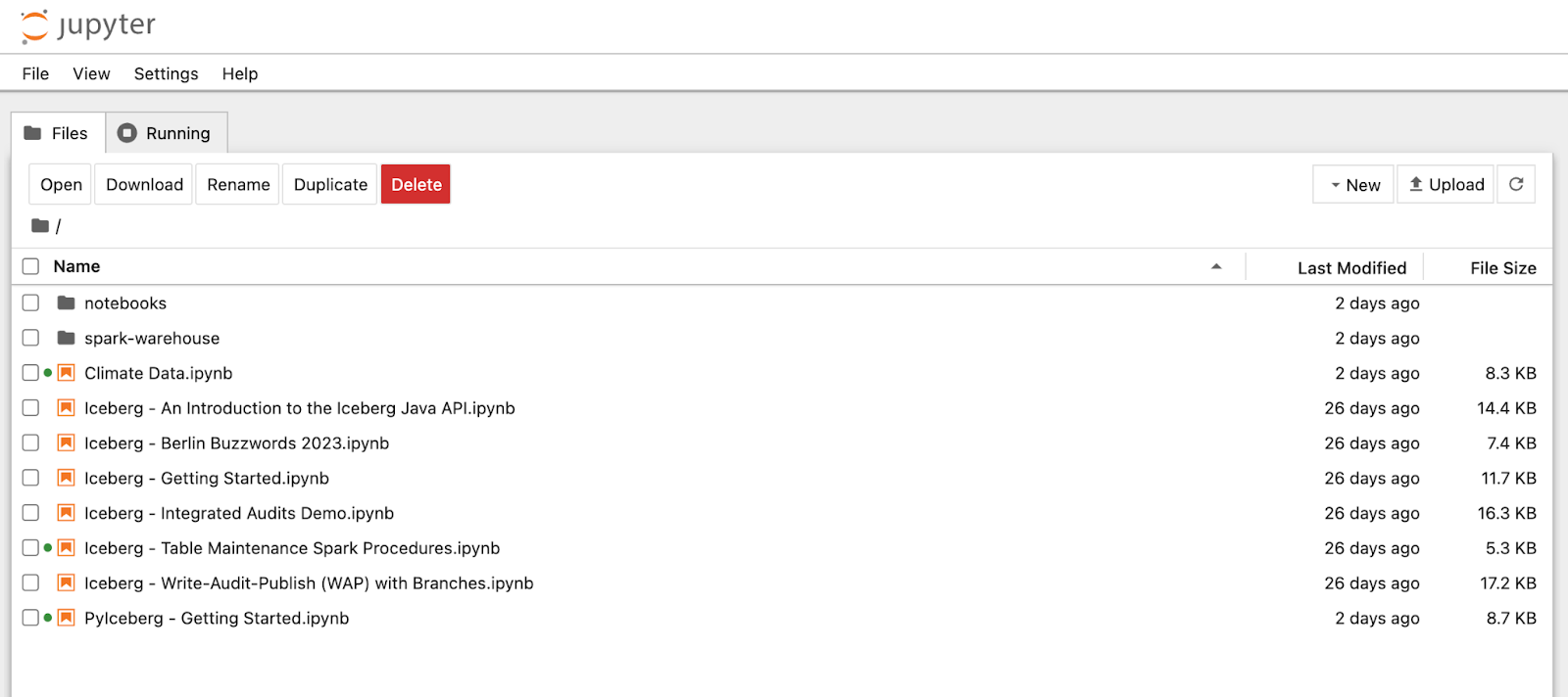
Once complete, navigate to localhost:8888. This is a port the Spark service exposes and it contains a Jupyter Notebook server. It should look like the screenshot below.

We are almost ready to create a table, insert data, and run queries. But before we do, let’s get an understanding of Iceberg’s data architecture.

Iceberg’s Data Architecture

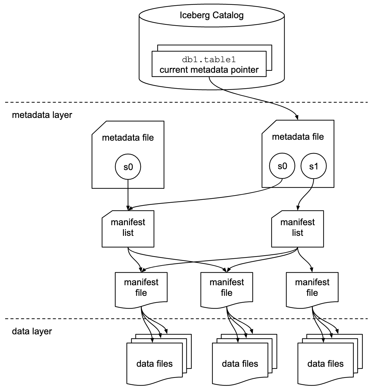
The diagram below from the Apache Iceberg specification best illustrates the different levels of metadata that are maintained by an implementation of Iceberg.

Source: https://iceberg.apache.org/spec/

Going through each of these levels is a good way to get a deeper understanding of Iceberg. As we go through each layer, keep in mind that the goal is to produce a design that allows for the easy implementation of the following capabilities:

• Schema evolution - Allow table designs to change without loss of data. In other words, add, drop, update, or rename columns.
• Hidden partitioning - Data architects should not have to create columns to allow a table to be partitioned. For example, adding a month column that is generated from a datetime field for fast retrieval of month-end reporting.
• Partition layout evolution - Over time, a table may experience unbalanced volume across partitions - or query patterns across partitions may change. There needs to be a way to modify the table layout (the partitions) to handle volume changes and query pattern changes.
• Time travel - Time travel is the ability to specify a date in the past as a part of a query and get a view of a table as it appeared on that date. Time travel enables reproducible queries on tables that are constantly updated. This is also important for machine learning workloads where you may need to see how a model was performing in the past. It is also a great way to create training sets and test sets.
• Version rollback - Allows a data architect to roll back a table to a previous state if a new design is bad or new data is corrupt or inaccurate.

If you have worked with relational databases, then you know that these design goals are a tall order.

Let’s conceptually go through each level of Iceberg’s data architecture to understand how Iceberg accomplishs the goals above. In the next section, when we create a table from scratch, we will look at actual metadata files to cement our understanding of these concepts.

Iceberg Catalog - The processing engine connects to the Catalog to get a list of all tables. For each table, the catalog keeps track of all Metadata files.

Metadata file (Level 1) - Contains schema and partition information. This could also include previous schemas and partitions if these were changed. The Metadata file also contains a list of snapshots. Every time a table is changed in any way, a new Metadata file is created based on the previous metadata file - the changes are placed in a snapshot and the new snapshot is added to the new Metadata file. Metadata files allow a table to be versioned and rolled back if necessary. They also contain the metadata needed for schema evolution, partition layout evolution, and hidden partitioning.

Manifest Lists (Level 2) - You can think of a single Manifest list as the snapshot itself - it provides a way to gather all the data for a given snapshot. Snapshots allow for time travel. In the diagram above, if you want the most recent version of the table, you would use the `s1` snapshot. However, if you wanted to use the table as it existed when the `s0` snapshot was created then you would use this snapshot.

Manifest Files (Level 3) - A Manifest file points to one or more data files. This is the part of the architecture that may seem unnecessary - but it is very important for efficient query execution. The Manifest file keeps track of which partition the data in a data file belongs to. It is this information that allows entire groups of files to be eliminated when a query is being planned. The Manifest files also contains column-level information pertaining to the values in each file. For example, if a column contains temperature readings, then the Manifest File will maintain max and min values for each Data File. This also facilitates efficient query planning.

Data Files - Finally, we get to the data. The Data Files contain the data. They are typically in Parquet format, but they could be any format the processing engine can parse.

I have made you wait a long time to code, but at least now you will understand everything that is happening under the hood as we create a table, add data to it, and then query the table.

For more on the overall architecture of Iceberg, check out The Definitive Guide to Lakehouse Architecture with Iceberg and MinIO.

Create a Table

Head on over to the Jupyter Notebook we installed earlier and create a new notebook. We will create a new database and a simple table that has one partition. To create the database put the code below in a cell. This will create a database named `climate.`

To create a table named `weather`, use the SQL below. This table has a partition that is by days.

Before adding data to this table, let’s take a look at what is happening within MinIO. After the command above completes, a Metadata file will be created - this is the first level of metadata in Iceberg’s data architecture. Open MinIO, which can be found at localhost:9001. Recall from the Docker Compose file that everything is going to the `warehouse` bucket. Drilling into this bucket, you should see something similar to the screenshot below. This is the metadata file for the weather table. Notice that the Rest Catalog is using the database name and table name as part of the path for this file.

This is the only metadata file that exists in MinIO at this point since we have not added any data to the table. We will open a metadata file once we have data.

Adding Data

The PySpark code below will add three rows to our newly created table. Notice that they are going to be in different partitions since the date falls on three different days.

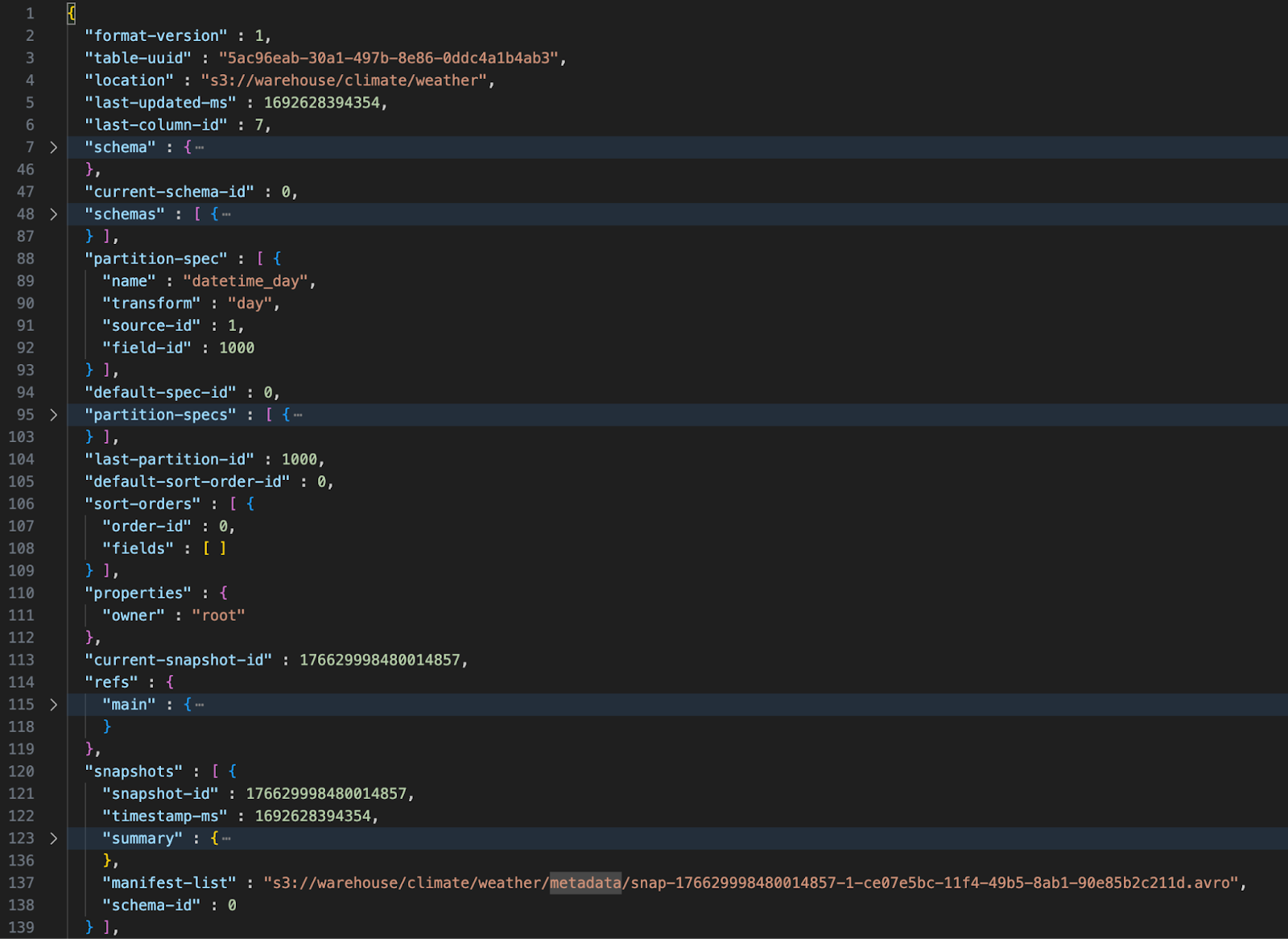
Now that we have data let’s open up the table’s metadata file. Below is an image showing the contents of the `weather` table’s metadata file after data has been added to the table. It is collapsed for brevity. Notice that it has placeholders for the current schema, the current partition, previous schemas, previous partitions, and snapshots. The current snapshot is pointing to a Manifest list file which is a point-in-time snapshot of this table.

Iceberg Metadata File - Level 1

The manifest list (or snapshot) is an Avro file. (Converting it to JSON can be tricky - use this website to do so - https://dataformat.net/avro/viewer-and-converter.) This file is shown below.

Iceberg Manifest List File - Level 2

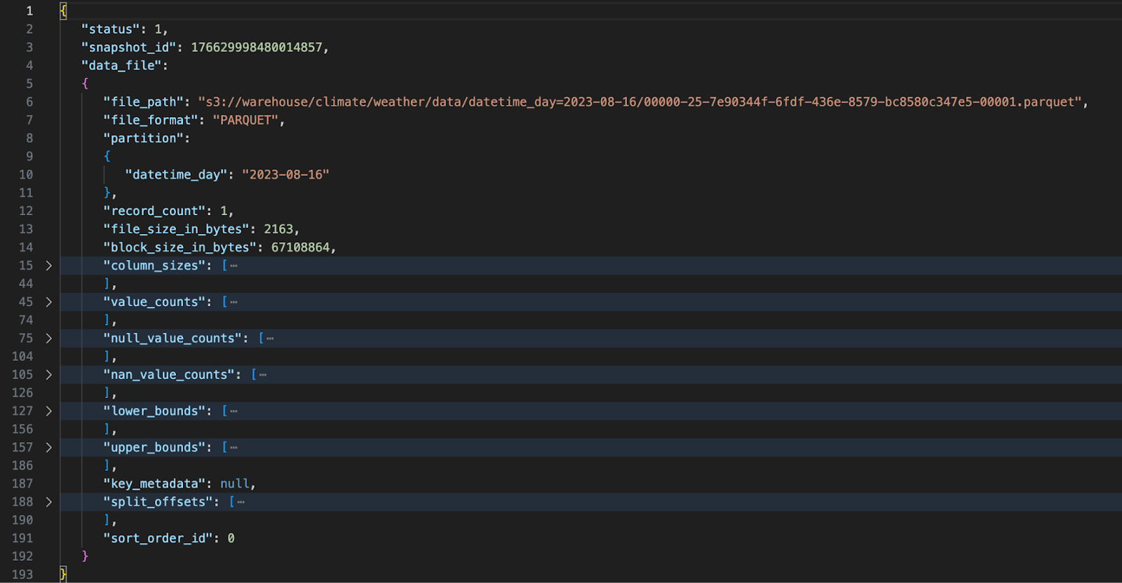
This is level 2 in the Iceberg data architecture. Manifest List files are relatively simple. Their main purpose is to keep track of a table’s state at a point in time. They do this by pointing to one or more Manifest files. In our simple example, we have only one Manifest file. Manifest files can get quite large - especially if your data is spread across many partitions. A collapsed portion of our Manifest file is shown below.

Iceberg Manifest File - Level 3

Manifest files represent the third and final layer in Iceberg’s data architecture. As such, they point to data files. Data files are usually in Parquet format and contain only data. Below is a screen shot showing the `data` path within the `warehouse` bucket.

Notice that there is a path for every partition needed thus far - we added data for three different days to a table partitioned by days. Organizing data files in this fashion is not a part of the Iceberg specification - it is an advantage you get when you use an object store like MinIO. Drilling into one of the partitions we can see the parquet files.

Now that we have some data in our Iceberg table, let’s conclude our developer investigation by querying the data.

Querying a Table

To show how easy it is to query data in Iceberg, I will use a fairly new Python library - PyIceberg. The promise of PyIceberg is to provide a way to query Iceberg tables without the need of a JVM. Unfortunately, at the time of this writing, PyIceberg can only be used for querying data - it cannot be used for adding, updating, or deleting data. Check the PyIceberg site for news pertaining to future developments.

PyIceberg is preinstalled in the Spark service we created via our Docker Compose file. The code below works when dropped into a new cell within our notebook. It will return all rows from the `weather` table that have a `datetime` field greater than or equal to August 1st, 2023.

The output will look like the image below.

Notice that this query takes advantage of the partition we created since we are filtering by the `datetime` field.

Summary

In this post, I presented a developer-oriented tour of Apache Iceberg. I showed how to use Docker Compose to get an implementation of Apache Iceberg running on a development machine. The implementation uses Spark for the processing engine, MinIO for storage, and a Rest Catalog. What is nice about the Rest Catalog I used is that it uses MinIO for Metadata. Other catalogs use distributed file systems or databases for Iceberg metadata - but this is not a modern solution and unnecessarily introduces an additional storage technology into the deployment. A better approach is to keep both metadata and data in high-speed, scalable object storage. This is what MinIO provides.  

I also presented Iceberg's goals and walked through Iceberg’s data architecture by creating a table and adding data to it. From there, I walked through the three levels of metadata that Iceberg maintains for every table. Finally, I presented PyIceberg - a new library for querying Iceberg data without the need for a JVM, which is needed for PySpark.

At MinIO, we love open table formats because they help set your data free and enable you to work with the latest cloud-native analytics and AI/ML frameworks.